Or Cohen

Regime Based Dynamic Asset Allocation - Part 2

Following the previous post, in this post we will learn how to incorporate regime predictions in our asset allocation models.

Statistics is the field of science that tells you that if your feet are in the oven and your head is in the freezer, on average, your body is fine. When it comes to asset management though, the variation of our subject, portfolio returns, is as important as its average; This is the core principal that guided 24-year old Harry Markowitz in deriving his Mean-Variance analysis, that was originally introduced in 1952 [1] and was since adopted by the vast majority of portfolio managers.

In essence, Markowitz devised an approach to portfolio selection that comprised two stages, forecasting and optimization, and identified the variance of returns as a critical measure of portfolio risk. His pioneering research established the foundation for understanding the power of diversification through the covariance between assets.

Mean Variance Optimization

Mean Variance Optimization (MVO) provides us with the optimal weight for every asset in our portfolio given the expected return and covariance of returns of these assets. Several variations and enhancements were developed based on its principals such as the Black-Litterman model that is a form of unconstrained MVO that incorporates investors subjective views (prior) on the expected returns of one or more assets.

In its original setup, the MVO formulation is as follows:

• \(\mathbf{r} = [r_1, r_2, \dots, r_n]^\top\) is the vector of expected returns for each asset,
• \(\Sigma\) is the covariance matrix of asset returns, where \(\Sigma_{ij}\) is the covariance between asset \(i\) and asset \(j\),
• \(\mathbf{w} = [w_1, w_2, \dots, w_n]^\top\) is the vector of portfolio weights (fractions of total capital invested in each asset),
• \(\mathbf{1}\) is a vector of ones (dimension \(n\)).

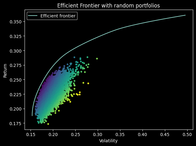
The objective is to maximize the expected return for a given level of risk \(\sigma_{target}\) , or equivalently, minimize risk for a given expected return \(r_{target}\). The expected portfolio return is given by:

The portfolio variance (i.e. proxy for risk) is:

And the formal optimization problem is therefor:

Where \(\lambda\) is a risk-aversion parameter that controls the trade-off between expected return and risk (note that it is not the same variable we used for jump penalty). A higher value of \(\lambda\) results in a more risk-averse portfolio.

In [1] the long-only and fully invested constraints were included which are defined formally as:

To solve this, we can use quadratic programming or other numerical optimization techniques. The resulting portfolio weights \(\mathbf{w}^*\) are those that maximize the objective function while satisfying the constraints. The optimal portfolio is determined by balancing the return and risk objectives, with the risk-aversion parameter \(\lambda\) controlling the degree of risk tolerance.

Putting the theory into practice

Markowitz acknowledged the challenge of accurately forecasting the returns of investment assets and recognized the need to incorporate additional methods and judgement in order to successfully implement his framework. The concept is brilliant but like other things in life, the proof is in the pudding. More accurate forecasts will enhance our investment performance and vice versa.

The forecasting signals from the JM-XGB [2] framework we viewed in the previous post can help us improve our forecast for asset class return given the predicted market-regime. For effectiveness and simplicity reasons, the regime forecasts are not used for covariance estimation.

As you know or may have guessed, there are several open-source code libraries that allow us to implement these models efficiently and backtest over long periods at lightning speed. PyPortfolioOpt is an extensive and efficient library for implementing portfolio optimization models.

import pypof

# exponentially weighted moving covariance matrix with a 252-day halflife
cov_matrix = pypfopt.risk_models.exp_cov(prices, span=252, frequency=252, log_returns=True)
# in-sample expected returns for the forthcoming predicted regime
expected_returns = JmXgbRegime.expected_returns
# construct efficient frontier model with 40% upper bound
ef = pypfopt.EfficientFrontier(expected_returns, cov_matrix, bounds=0.4)
# add 1% broker commission
ef.add_objective(pypfopt.objective_functions.transaction_cost, w_prev=current_weight, k=0.01)
# computre weights that maximize quadratic-utility given the risk aversion (lambda = 10)
weights = ef.max_quadratic_utility(risk_aversion=10)
# show the expected portfolio performance
ef.portfolio_performance(verbose=True)

We can follow the article setup as demonstrated in the code above or specify our target risk or target return with the efficient_risk and efficient_return functions. For reproducibility purposes, I wrapped the JM-XGB framework detailed in the previous post within a python class JmXgbRegime that upon fitting to historic data provides the expected returns given its prediction for the forthcoming market regime for each asset class.

PyPortfolioOpt also provides more advanced optimization models, for example optimizing along the efficient mean-semivariance frontier which instead of penalising volatility seeks to only penalise downside volatility.

Backtest Results

To evaluate the added value of incorporating the market regime signal in the asset allocation decision process, the researchers compared the performance of three allocation methods both with and without the regime signals.

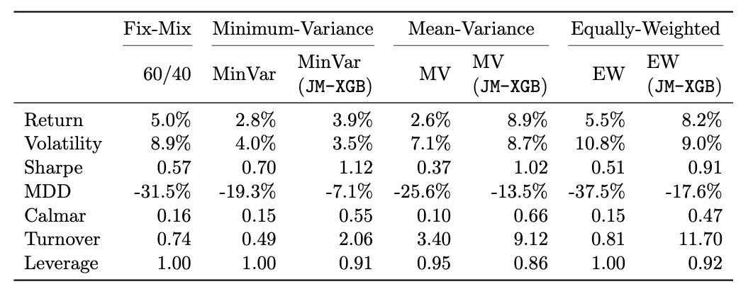Annualized performance metrics for each allocation method tested between 2007-2023. A 60/40 allocation between equity, real-estate, high-yield and commodities (60) and the three-bonds indexes (40) was added as a benchmark. Source: [2]

Evidently, the market regimes signal improved every allocation method and generated higher returns with lower downside risk. This dual sided improvement highlights the appeal of this framework to a wide range of investors with different risk aversion characteristics and investment objectives. The wealth curves below showcase the consistent outperformance of the enhanced asset allocation version of all methods.

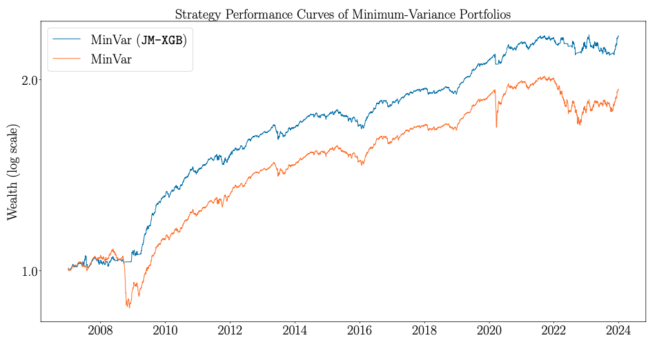
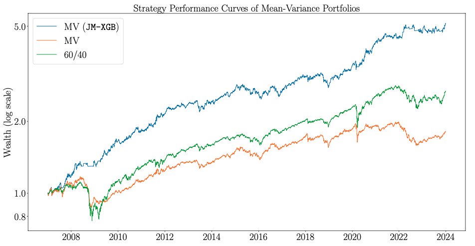
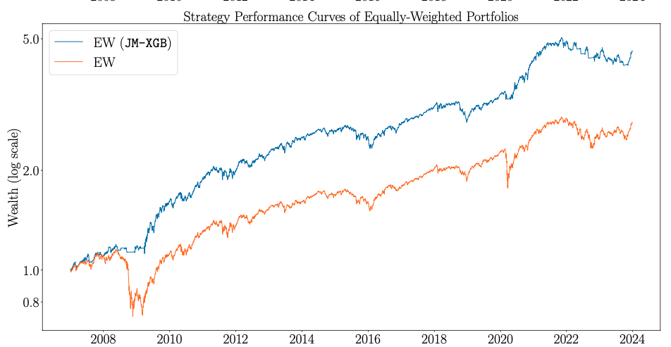Wealth curves of the JM-XGB enhanced vs. standard allocation method. Source: [2]

Conclusion

Diversification is known to be the only free-lunch in investing and the corner-stone of sound portfolio management. The effect of an adaptable approach to asset allocation is substantial yet largely dependent on the portfolio manager’s ability to form accurate return expectations for every asset class.

A taw-aware implementation of this strategy can also increase our net return and generate a tax-alpha. In the most basic level it entails switching the ETFs that are used to track an index upon an end of a bear regime to lower the coast basis.

As always, please don’t hesitate to send me any feedback, questions or suggestions you have!

References:

1. Markowitz, H.M. (1952). Portfolio Selection, The Journal of Finance.
2. Shu, Y. (2024). Dynamic Asset Allocation with Asset-Specific Regime Forecasts, Annals of Operations Research.