Or Cohen

Regime Based Dynamic Asset Allocation - Part 1

In this post we will find out how market regimes forecasts can help us to improve our portfolio asset allocation. If you haven’t read the previous post about Statistical Jump Model (SJM), I recommend starting there.

Since my service in the Israeli Navy I’m hooked on sailing and exploring the seas. One basic truth that all sailors know is that although you can’t control the wind, you can adjust the sail. This simple notion is also true for our portfolio management.

It is well known that asset allocation is one of the greatest determining factors of our investment outcomes. Academic studies that were published over the past three decades tried to asses to what extent portfolio performance of active managers in pension funds was attributed to investment strategy (security selection and market timing) versus investment policy (asset allocation). The conclusions of these studies leaned heavily towards policy but initiated a debate and several follow-up studies.

Prof. Meir Statman in his article [1] provided a thoughtful mediation to the claim that investor management (i.e. the role of a financial advisor in advocating for a disciplined investment policy) is more important than investment management (security selection and tactical asset allocation). His conclusion was that tactical asset allocation based on perfect foresight performed 8.1% better per year during the eighteen years 1980-1997, yet the strategic asset allocation still explained 89.4% of the variance.

In other words, Statman conclusion was that strategic asset allocation is movement along the efficient frontier, whereas tactical asset allocation involves movement of the efficient frontier. Statman study was deliberately hypothetical since no one has perfect foresight but proves that if as investors we adjust the sail we may get a little stronger push from the wind.

Between the the two approaches [1] compared (strategic vs. tactical asset allocation) exists dynamic asset allocation (DAA). In DAA, we alter the weights of the various asset classes in our portfolio based on the prevailing market conditions. In this way, we still benefit from diversification by allocating to different asset classes but limit the downside risk by avoiding sustained periods of declines.

As always, we should consider the risks and limitations which are mainly the transaction costs that are associated with higher turnover in our portfolio and the possibility of wrong forecasts the can eventually lead to losses rather than gains. This leads us to the understanding that the proof is in the pudding - DAA can have a sustained positive impact on our investment performance, if we have good predictions on the market.

Predicting Market Regimes

Shu et al. introduce in their research [2] a hybrid framework that on a high level augments asset allocation methods, such as mean-variance optimization, with asset-specific return and risk forecasts. These forecasts are derived using a sophisticated model that is based on a binary regime prediction (Bull or Bear) and are used to determine the optimal asset allocation weights.

Since market regimes are latent states, identifying and labelling them is a prerequisite for training a classification model that predicts the forthcoming regime based on historical data. At first, this may seem unnecessary since our premise is that market regimes are persistent and thus the identification model can suffice. In practice, separating the task of forecasting regimes to identification and prediction stages allows us to employ a specialized model for each step.

The novel hybrid identification-forecasting approach proposed in [2] delivers better out-of-sample forecasting results than other variants of HMM based forecasting. In essence, it couples the SJM [3] described in the previous post with a boosted-trees classifier, XGBoost, via a cross-validation (CV) hyper-parameter optimization for the jump penalty factor λ that aims to maximize Sharpe ratio.

Implementing this framework requires a fair share of engineering but in return delivers a robust and performant forecaster that can significantly ameliorate our asset allocation and risk management. Let’s have a look at the practical steps to understand it better.

Assets Universe and Feature Engineering

The researchers in [2] selected 13 asset classes that are commonly used by allocators as the investable asset universe. The python dictionary below indicates the corresponding ETF that serves as a proxy for the chosen index for that asset class.

assets = {
	'large_cap':'SPY',
	'mid_cap':'IJH',
	'small_cap':'IWM',
	'eafe':'EFA',
	'em':'EEM',
	'aggbond':'AGG',
	'treasury':'SPTL',
	'high_yield':'VWEHX',
	'corporate':'LQD',
	'reit':'IYR',
	'commodity':'GSG',
	'gold':'GLD'
	}
risk_free_rate = get_fred_data(series='TB3MS', frequency='m')

This asset class universe offer extensive diversification across macroeconomic factors and various countries, including both developed and emerging markets, and span all the major assets used by traditional allocators: equities, fixed income, real estate, and commodities.

For the first stage of the framework, classification to regimes using the continuous SJM, the set of features will be derived from the historic daily excess returns (i.e. over the risk free rate) of each asset. These features are the EWMA of raw-returns, log-drawdown and Sortino ratio across 3 different half-life values: 5,10,21. We get the Sotrino ratio from the division of the EWMA return by EWMA log-drawdown for the same half-life value. In essence, these features capture the recent excess returns, down-side risk and down-side risk adjusted returns for each asset.

For the regime forecasting in the second stage we use the same asset-class specific set of features described above along with a set of five macro features that are common to all assets. The first macro feature is the one month trend of the 2-year yields, which uncovers whether interest rates are in a rising or falling trend. The yield curve slope and its trend, the second and third features, are well known as the most powerful predictors of future economic growth, recessions and inflation and are widely watched by investors.

# Download yields from FRED API
yields_df = pd.DataFrame({
	'2y': get_fred_data('DGS2','d'),
	'10y':get_fred_data('DGS10','d')
	}).assign(spread= lambda x: x['10y'] - x['2y'])

vix = yf.Ticker('^vix').history(period='max').Close.apply(np.log)
 
macro_features = pd.DataFrame({
	'2y_trend': yields_df['2y'] - yields_df['2y'].ewm(halflife=21).mean(),
	'YC_slope': yields_df['spread'].ewm(halflife=10).mean(),
	'YC_trend': yields_df['spread'] - yields_df['spread'].ewm(halflife=21).mean(),
	'VIX_trend': vix - vix.ewm(halflife=63).mean(),
	'eq_fi_corr' : data['SPY'].rolling(window=252).corr(data['AGG'])
	})	

The VIX index is a forward-looking volatility estimator for the next 30-days based on the prices of options on the S&P500. We calculate its smoothed trend to gauge the anticipated equity risk by market participants. Lastly, the correlation of stocks and bonds is often falling during a recession or an economic crisis due to the “flight to safety” phenomenon, and on the other hand, a positive correlation is observed during periods of economic growth and low interest-rates in which investors confidence is high.

Coupling Identification and Forecasting Models

On this foundation of the two models we can develop the training loop. On every training iteration we use an 11-year lookback window and a given λ value to: (1) fit a SJM to generate regime labels with the returns based features, (2) fit an XGBoost classifier for the labels with the expanded features set , and (3) generate daily regime forecasts for the next six-months.

def algorithm1(X1, X2, returns, jump_penalty, pred_start, pred_end):
    biannual_windows = pd.date_range(start=pred_start, end=pred_end, freq='6MS')
    predictions = []
    for date in biannual_windows:
        lookback_window = slice(date - pd.DateOffset(years=11), date)
        prediction_window = slice(date, date + pd.DateOffset(months=6))
        jm = JumpModel(n_components=2, jump_penalty=jump_penalty, cont=False)
        # fit jump model
        jm.fit(X1.loc[lookback_window], returns.loc[lookback_window], sort_by="cumret")
        # make labels
        regime_labels = jm.predict(X1.loc[lookback_window])
        # merge asset class specific features with macro features
        predictors = X1.merge(X2,left_index=True,right_index=True, how='left')
        # fit xgboost
        forecaster = XGBClassifier(objective='binary:logistic', eval_metric='logloss')
        forecaster.fit(predictors.loc[lookback_window], regime_labels)
        # predict the probability fot the forthcoming half year
        preds = forecaster.predict_proba(predictors.loc[prediction_window])
        preds = pd.Series(preds[:,1], index=predictors.loc[prediction_window].index)
        predictions.append(preds)
    return pd.concat(predictions).apply(lambda x: 1 if x > 0.5 else 0)

The above depicted steps are repeated every six months for a given prediction window and λ value for each asset class. As we know, the jump penalty factor λ is a critical hyper-parameter that directly affects the accuracy of the classifier. Its fine-tuning is the interesting part where the researches deployed a CV optimization method based on the financial outcome rather than on a statistical measure of classification such as ROC-AUC.

To asses the financial performance of algorithm 1, we will calculate the Sharpe Ratio of a regime switching strategy termed “0/1 strategy” [4] based on the predictions of algorithm 1 for a range of λ values. The 0/1 strategy is a just simple binary strategy that alternates between 100% investment in the risky asset and a 100% investment in a risk free asset.

The researchers chose to use a five-year window for the CV part, meaning that during a five-year window we biannually call algorithm1 and compute the Sharpe Ratio for the 0/1 strategy during that period. We then select the λ value that yields the highest Sharpe Ratio across all 10 periods (5 years X 2) to generate the out-of-sample (OOS) forecasts for the next six-months.

def algorithm2(jump_penalties, test_start, test_end, asset_returns):
	biannual_windows = pd.date_range(start=test_start, end=test_end, freq='6MS')
	best_jps = dict()
	for cv_end in biannual_windows:
		sharpe_per_jp = dict()
		for jump_penalty in jump_penalties:
			cv_start = cv_end - pd.DateOffest(years=5)
			cv_window = slice(cv_start, cv_end)
			# forecast regimes for the cv period
			regime_preds = algorithm1(X1, X2, cv_start, cv_end)
			# apply the 0/1 strategy based on the predicted regimes
			zo_strategy = np.where(
					regime_preds == 1,
					risk_free_rate.loc[cv_window],
					asset_returns.loc[cv_window]
					)
			# calculate the Sharpe ratio
			sharpe_per_jp[jump_penalty] = zo_strategy.mean() / zo_strategy.std()
		# save the jump penalty that maximized Sharpe during the cv period
		best_jps[cv_end] = max(sharpe_per_jp, key=sharpe_per_jp.get)
	return best_jps

To summarize, we use 11 years of historic data for training the hybrid model and 5 years of historic data for the CV tuning of λ, so that’s a 16 years history of daily returns in total. This distinction between the training and validation periods is a clever design choice that simulates a live setting and ensures more robust OOS predictions.

In addition, this way of linking the classification and forecasting achieves a synergy between the models used in the both stages and provides us with a tailored, financially-optimized regime forecasting model for each asset class.

Outcomes

Observing the model results provide us several practical conclusions and considerations. For a complete comparison of the hybrid approach (JM-XGB) with the buy and hold strategy and JM alone see the table at the end of this section.

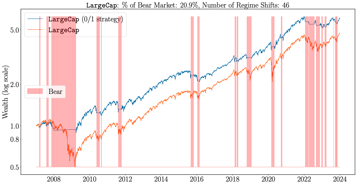
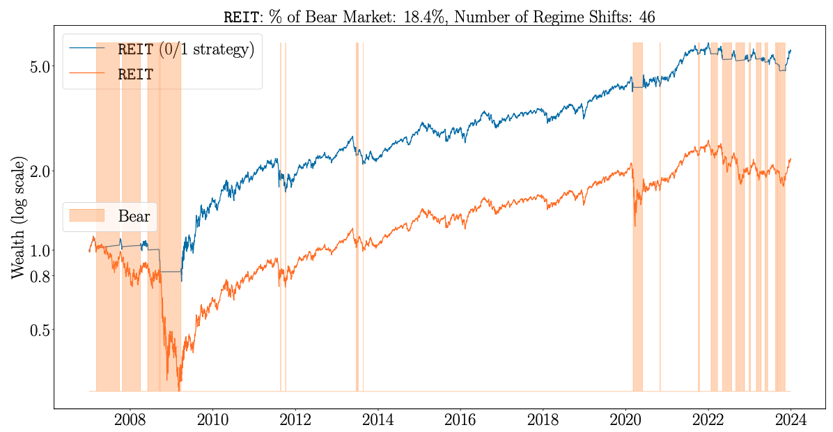
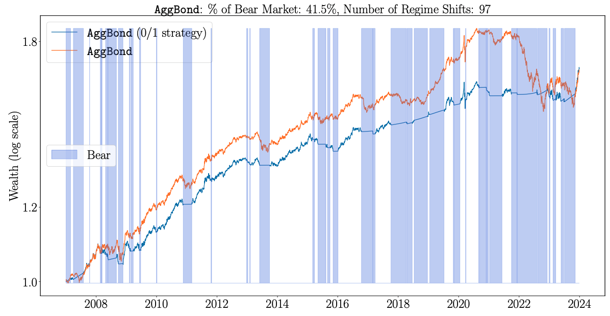Regime forecasts of JM-XGB for LargeCap stocks, REITs and the US AggBond index. Source: [2]

A birds eye-view of all three proves that the optimized market regime forecasts are distinct to each asset class and hence a tailored model for each is preferable. For instance the early impact that the subprime mortgage crisis had on REITs is reflected in the earlier bearish regime forecast for REITs compared to LargeCaps.

It is also noticeable that the forecasted bearish regimes capture all major market downturns including the global financial crisis, the Covid crash of 2020 and the interest rate hikes in 2022 that affected the AggBond index and increased the volatility of other assets.

One noticeable challenge for the model is evident by the bearish forecasts for AggBond which constitute 42% of the periods, considerably higher than the 21% for LargeCaps and 18% for REITs. According to the research, this is a result of creating features based on excess returns since during periods of high interest rate the excess return of AggBond is diminished. The higher Sharpe Ratio of the buy-and-hold strategy on Gold (see table below) is another evidence of that issue.

Another challenge, that in a way is here to stay, is the delay of forecasts evident by several bear regime forecasts that lagged significant drops; for example during the 2015-2016 market selloff for LargeCaps as result of Brexit, the Greek debt default and the Chinese stock market turmoil. With that, until we find that crystal ball, this model proves significantly better than the buy-and-hold strategy.

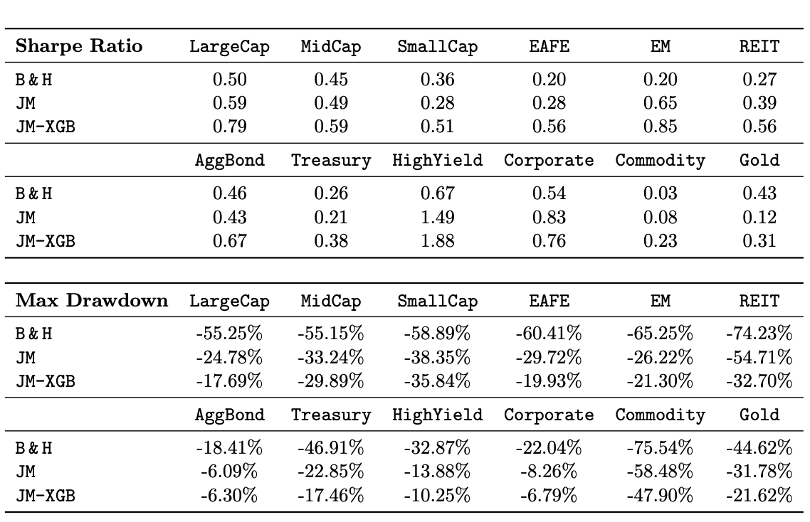Performance metrics for the 0/1 strategy applied to individual assets vs. buy & hold, between 2007-2023. A one-way transaction cost of 5 basis points was applied. Source: [2]

Midpoint Conclusion

The outcomes in the table above prove the power of incorporating market regimes in our risk and portfolio management, even when used only as a simple kill switch (0/1 strategy). It is particularly effective for mitigating the downside risk as evident by the lower maximum drawdown across all asset classes.

In the next post we will see the benefits of incorporate the regime forecasts in our asset allocation decision making process.

References:

1. Statman, M. (2020). The 93.6% Question of Financial Advisors, The Journal Of Investing.
2. Shu, Y. (2024). Dynamic Asset Allocation with Asset-Specific Regime Forecasts, Annals of Operations Research.
3. Nystrup, P. (2020). Learning hidden Markov models with persistent states by penalizing jumps, Expert Systems with Applications.
4. Bulla, J. (2011). Markov-switching asset allocation: Do profitable strategies exist?, Journal of Asset Management.