Change Point Detection with Statistical Jump Models
![]()
In this post we will explore the benefits of identifying regimes in financial markets and learn how to statistically classify and predict change points in regimes.
The German philosopher Georg Hegel said: “The only thing that we learn from history is that we learn nothing from history”. History repeat itself in almost every aspect of our lives and financial markets are no different. One valuable insight we can gain from studying the history of financial markets is the prevalence of common patterns that repeat in the evolvement of asset prices.
The cyclical regime switching behavior of asset returns is well-documented across various asset classes, including equities, fixed income, commodities, currencies, and cryptocurrencies.
Market regimes are essentially clusters of persistent conditions that affect the returns of different asset classes and the relevance of investment factors. The change of these regimes is usually a result of a change in the macroeconomic environment, e.g. a change in inflation or unemployment levels.
Fundamental macro indicators are often discovered retrospectively while the dynamic nature of markets reflects their influence concurrently. Early change point detection (CPD) of market regimes is a valuable input to strategic investment decisions such as asset allocation and the level of exposure to various investment factors. However, the stochastic nature of prices means that identifying a persistent change is a challenging task given the low signal to noise ratio.
Demystifying The Black Box
One common argument often raised by active asset managers when it comes to applying machine learning models in the investment process is that these models are hard to understand and are not grounded in fundamental economic theory. In reality, this is far from the truth.
A scientific approach to asset management can help us uncover insights that are hard to observe in financial data and also commit in advance to a disciplined and objective decision making approach that will protect us from our biases. Notwithstanding experience and human judgement are irreplaceable.
All the lengthy statement above is to say that before we decide to include a quantitive method in our toolbox we should confirm our ability to both understand and evaluate the quality of its outcomes with expert knowledge. This is especially true in the case of CPD giving the pivotal (pun is intended) role it has in our strategic decision making.
Hidden Markov Models and Statistical Jump Models
We know that market regimes are clusters of persistent conditions that are not directly observable from the data. A large body of research was dedicated to the improving the application of Hidden Markov Models (HMM) to CPD.
A Markov process is a random process in which the future is independent of the past, given the present. In the case of a discrete state the Markov process is known as Markov chain. In an HMM, the probability distribution that generates an observation depends on the state of an unobserved Markov chain.
The application of HMMs for CPD is prone to several errors that stem from the challenge in correctly specifying their parameters and result in an unstable and impersistent estimates of the underlying state sequence. Statistical Jump Model [1] (SJM) is a novel approach for learning of HMM parameters and is particularly interesting due to its interpretability and ability to control the state transition rate via a regularization factor λ.
The advantage of controlling the state transition rate when incorporating HMMs in our investment strategies lies in the need to balance the turnover rate. In the absence of ground truth for the labeling of state sequences, we can use our knowledge of investment strategies to fit the model in a way that maximizes the risk adjusted return and reduces the transactions costs associated with high turnover.
An extension to the SJM learning approach in [1] is the Continuous Jump Model (CJM) [2] that turns the discrete hidden state variable to a probability vector over all regimes. This provides a smooth transition between regimes that is both more robust and applicable for investment decision making.
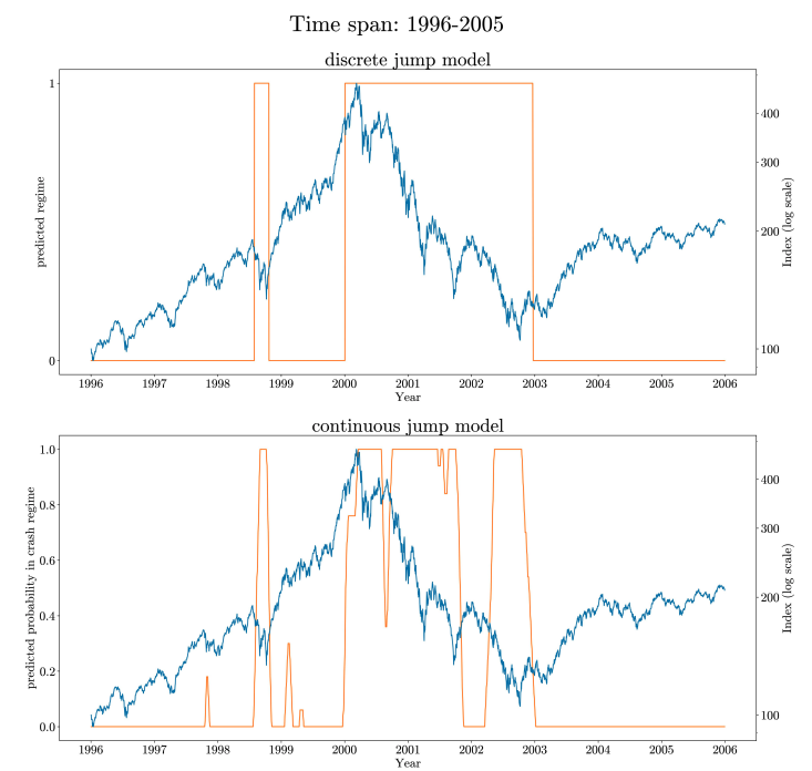 Bear (1) and Bull (0) regime predictions (yellow) of the Nasdaq Index (blue) using discrete and continuous Statistical Jump Models. Source [1].
Note in the Nasdaq comparison above that while the discrete model identifies the dot-com crash as a single bear period, the continuous one is able to detect two rebound periods with a smoothed transition.
Tuning SJMs
Alongside the scientific contribution, the research teams behind the two models also contributed to the open-source community by providing a well documented python library of SJMs. The key to successful integration of the model to portfolio and risk management lies in fine-tuning the jump penalty parameter λ through cross-validation or a statistical criteria (similar to a loss function).
This hyperparameter serves as a control dial for the fixed-cost regularization term associated with transitions between different states. In other words, its value reflects our prior assumptions about the frequency of state transitions.
jump_penalty=50
# initlalize a JM instance (set the arg cont=True for CJM)
jm = JumpModel(n_components=2, jump_penalty=jump_penalty, cont=False)
# fit data
jm.fit(X_train_processed, log_ret, sort_by="cumret")
# make online inference
labels_test_online = jm.predict_online(X_test_processed)
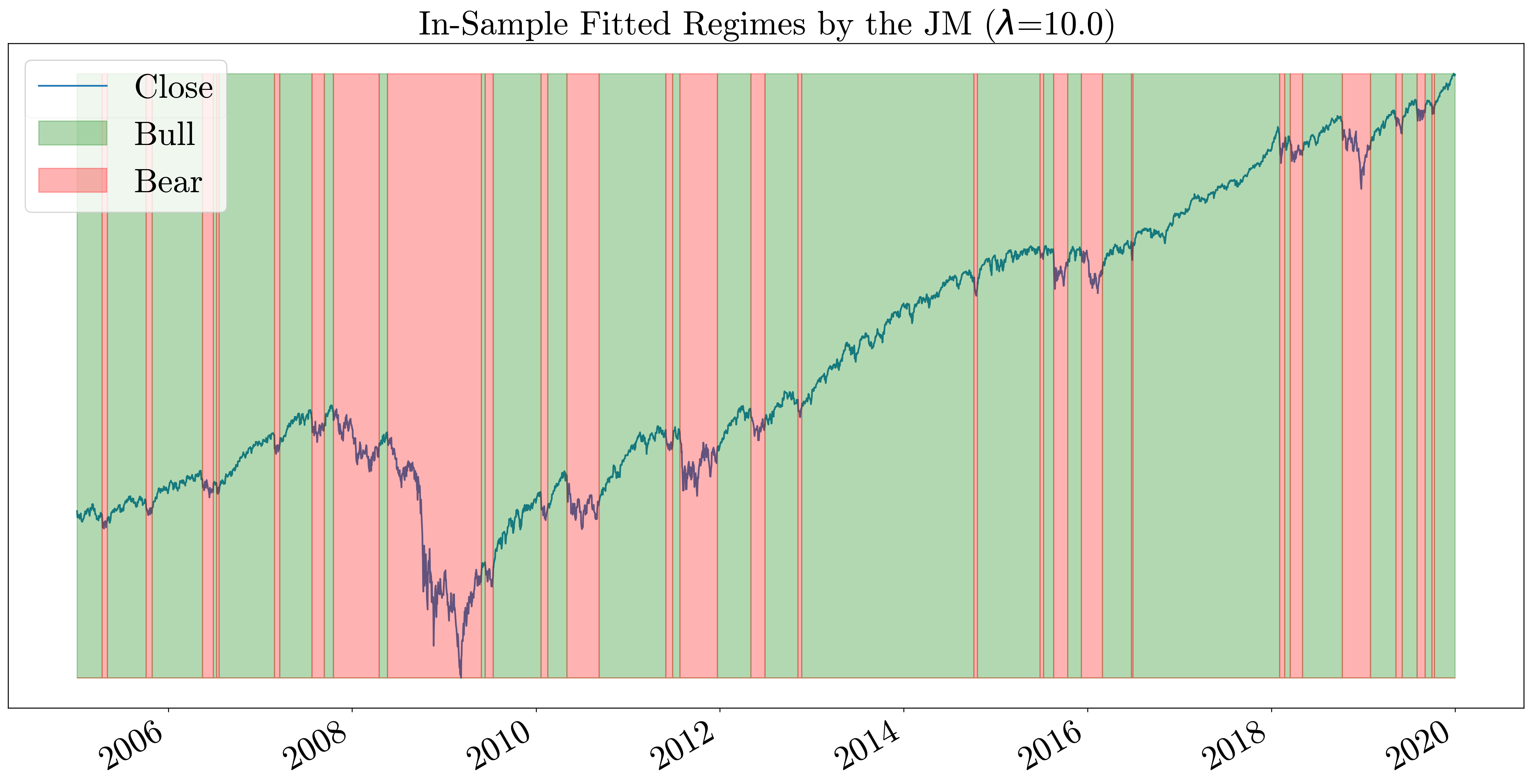
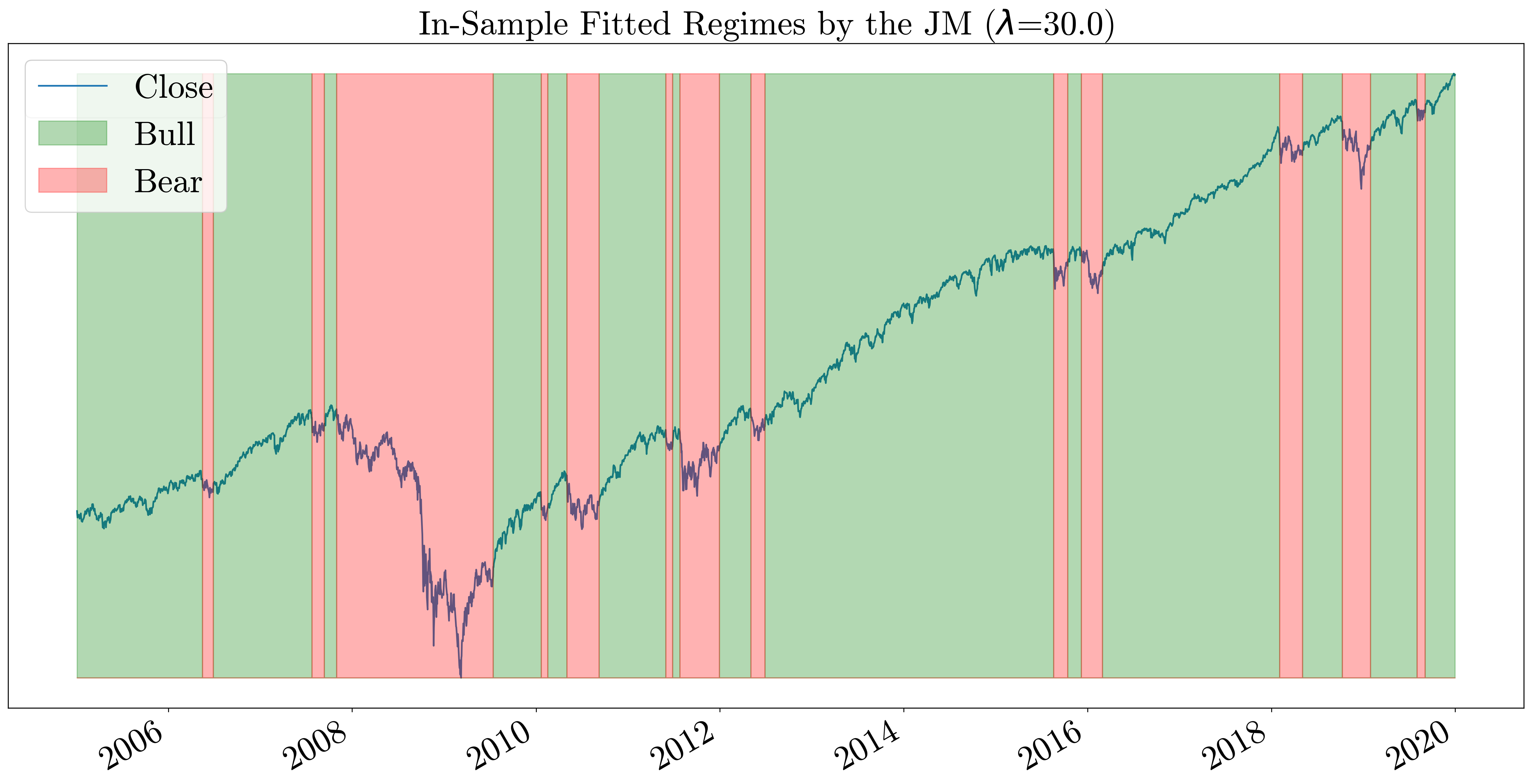
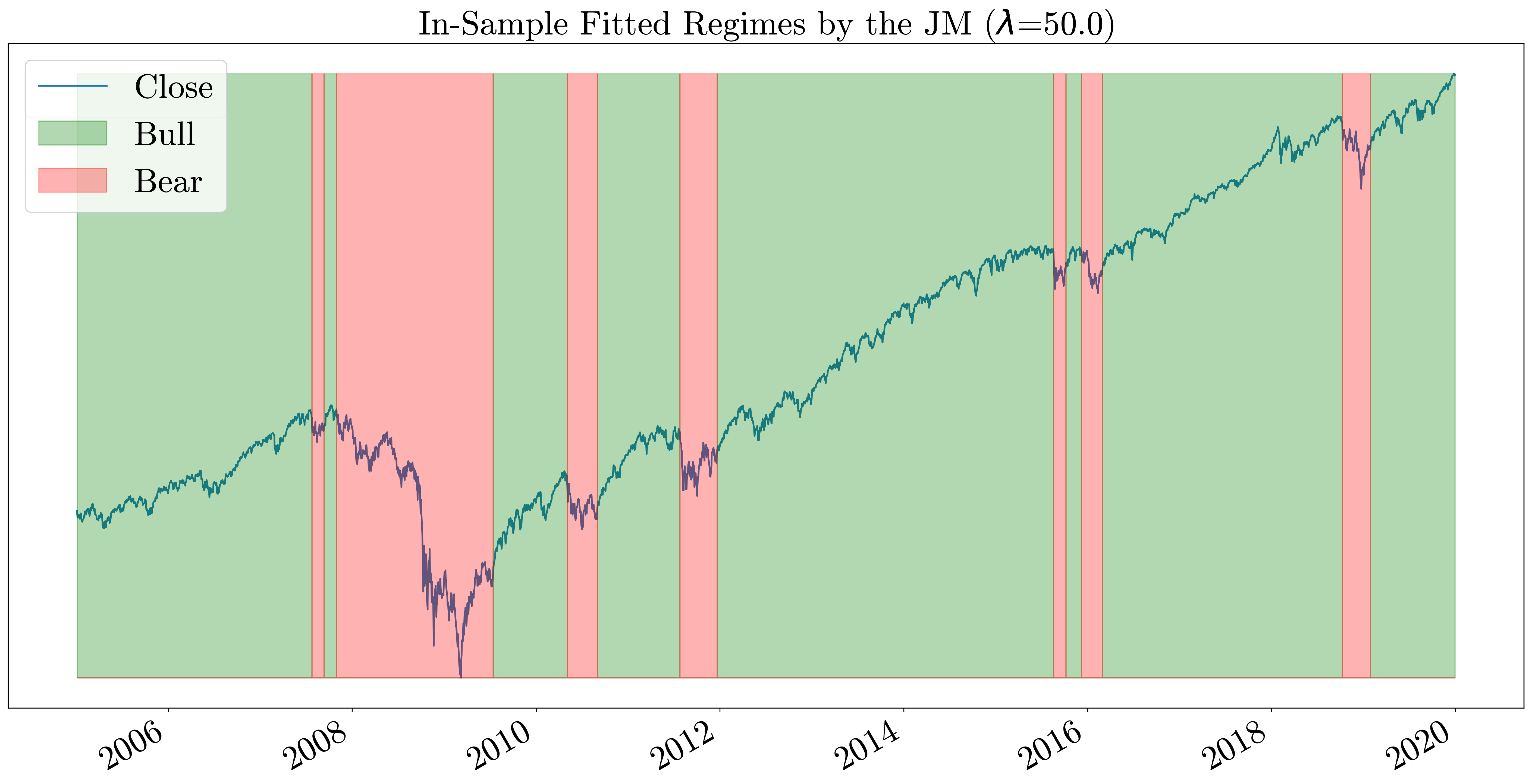
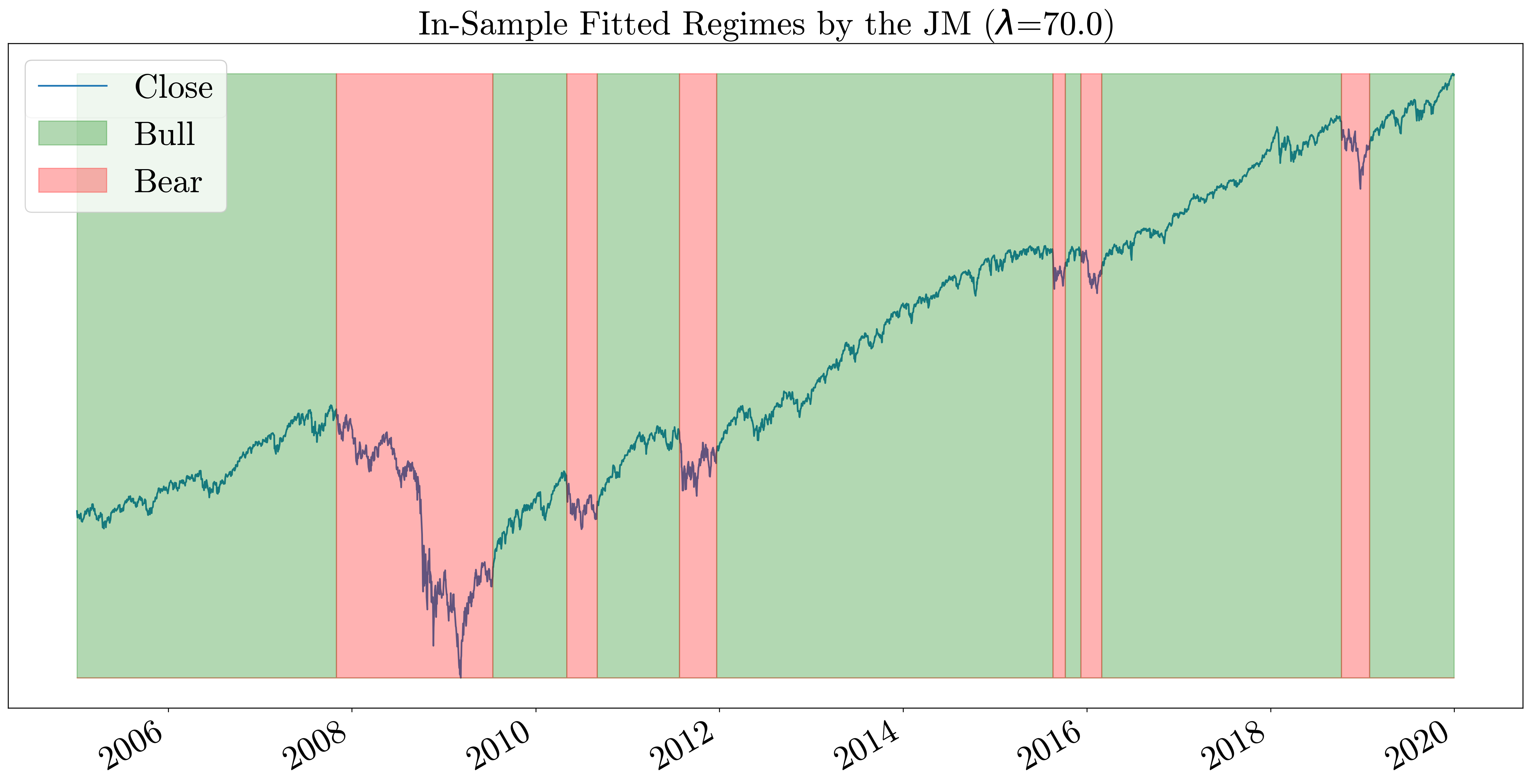
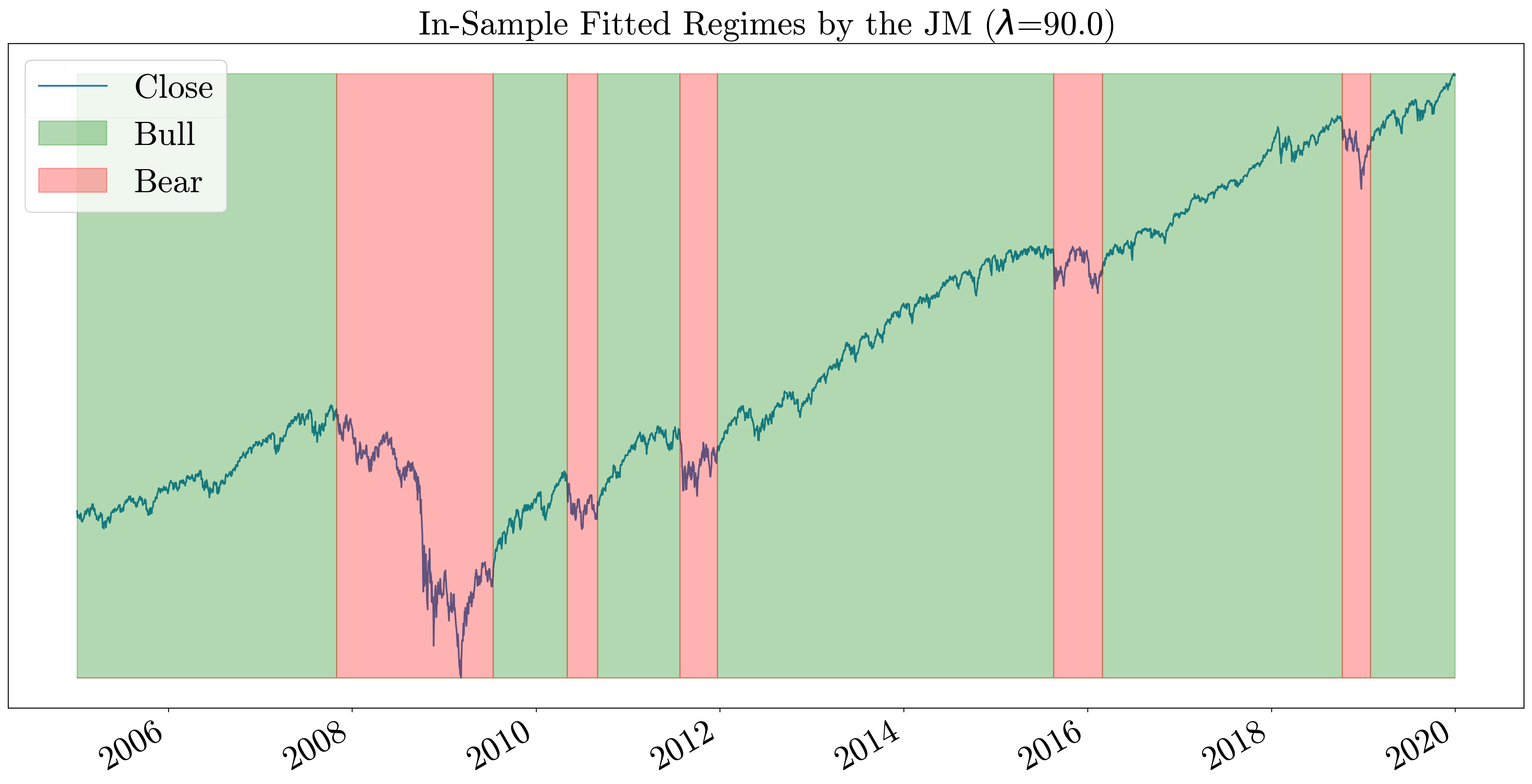
When λ is set to zero, the jump model becomes the K-means algorithm which does not take the temporal order into account. As we increase the value of λ, the number of state transitions decreases. In the plots below we can see the difference between in-sample fitted regimes by the model on the S&P500 index between 2005-2019 for λ values 10, 30, 50, 70, 90.
Conclusion
Time series clustering is a powerful technique for analyzing temporal data that we can use to adapt our strategies to the changing dynamics in financial markets. In the next post we will build upon this knowledge and learn how to improve our strategic asset allocation based on the insights this models provide us.
References:
- Nystrup, P. (2020). Learning hidden Markov models with persistent states by penalizing jumps, Expert Systems with Applications.
- Aydınhan, A. O. (2024). Identifying patterns in financial markets: Extending the statistical jump model for regime identification, Annals of Operations Research.