Or Cohen

Profit-Sensitive ML Credit Risk Models - Part 2

Following the previous post, in this post, we will explore how to enhance the business applicability of an XGBoost classifier by incorporating cost data into its learning process.

I recently watched the BBC series Rogue Heroes, which tells the story of the early years of the SAS. This unit’s story and motto have inspired not only other military forces but also professionals in various fields. What struck me most was their ability to learn by doing and succeed by taking calculated risks. In that spirit, and without undermining the incredible contributions of these courageous individuals, let’s adopt a similar approach in the credit domain and examine how taking greater risks can lead to higher profitability.

Problem Context

Let’s assume our goal is to advise a senior bank manager interested in investing in the P2P lending market. The manager’s objective is twofold: to deploy as much capital as possible while maximizing profits. As we learned in the previous post, machine learning can be a powerful tool for this purpose. We will experiment with different models using the Lending Club dataset.

You can follow along and execute the code by opening the Jupyter notebook linked above in Google Colab. To keep this post concise, we will focus primarily on Parts 3 and 4, as the first two sections cover basic concepts. At the end of Part 2, we observe that XGBoost’s ability to address imbalanced classification by assigning greater weight to the minority class significantly improves its forecasting performance based on statistical measures. However, since our goal is profit maximization while deploying as much capital as possible, we need a metric to compare the profitability of each loan.

Deriving Profitability Scoring

Several metrics can be used to assess loan profitability, such as internal rate of return (IRR), *annualized rate of return (ARR), and return on investment (ROI). IRR is best suited for comparing fully paid, prepaid, and defaulted loans. However, since the Lending Club dataset does not provide monthly records for each loan, deriving IRR requires multiple heuristics. The most straightforward approach is to estimate the total gain or loss for each loan over its lifetime.

One key consideration is prepayment risk. When borrowers prepay their debt, the lender loses the interest income for the remaining term of the loan. Accurately estimating prepayment risk requires additional models. For simplicity, we will assume perpetual reinvestment opportunities—meaning that when a borrower prepays a loan, the capital is immediately reinvested into a loan with an identical profile.

The dataset contains both 3-year and 5-year loans, making the total profitability of 5-year loans naturally higher. Additionally, defaulted loans tend to have shorter lifespans than fully repaid loans. To enable a fair comparison across all loans, we will calculate the total profit for fully paid loans over the average life of defaulted loans, which is approximately 17 months.

\(Profit_{TN} = \frac{(\text{Monthly Installment} \times \text{Avg. Life}) + \text{Prepayment Amount}}{\text{Loan Amount}}\)

avg_life = df.query('default').tenure.mean()

# Expected outcome of correctly predicted good loans
df['installment'] = df.loan_amnt * \
    (df.int_rate.div(12) * df.int_rate.div(12).add(1).pow(df.term)) \
    .div(df.int_rate.div(12).add(1).pow(df.term).sub(1))

df['exp_total_pymt'] = df.installment.mul(avg_life) + \
    (df.loan_amnt * ((df.int_rate.div(12).add(1).pow(df.term) - \
    df.int_rate.div(12).add(1).pow(avg_life)) \
    .div(df.int_rate.div(12).add(1).pow(df.term).sub(1))))

df.loc[~df.default, 'pi_tn'] = df.exp_total_pymt.div(df.loan_amnt)

For defaulted loans, the Lending Club dataset includes the recovery amount, which represents the funds lenders manage to recover after default. Since the collection process begins only after 150 days past due and can take months, the time value of money must be considered. To properly reflect the loss, we will discount the recovered amount using the present-value formula, assuming it is received approximately two years after the last payment date. Many financial institutions use the loan interest rate as the discount rate, though a less conservative approach would be to use the risk-free rate.

# Outcome of incorrectly predicted good loans
df['recoveries_pv'] = df.recoveries.div(df.int_rate.add(1).pow(2))
df.loc[df.default, 'pi_fn'] = df[['total_rec_prncp', 'total_rec_int',
                                  'recoveries_pv', 'total_rec_late_fee']].sum(axis=1).div(df.loan_amnt)

Comparing Profitability of Loans

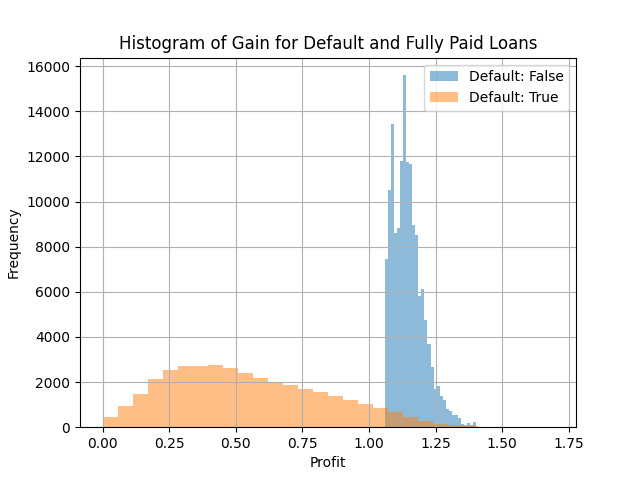
From the plot below, we observe a wide distribution of gains from defaulted loans, with some defaulted loans even outperforming certain fully paid loans. This occurs because loans that default late in their term may still generate substantial returns.

To compare the ability of our baseline models to select profitable loans, we will evaluate two methods for setting the decision threshold:

1. Selecting loans with the lowest probability of default (PD) as predicted by the model.
2. Using the default premium (from the previous post) to select loans with the greatest spread between the interest rate and default premium.

Note that in both cases, we will select the top 80% since we know that the default rate is about 20%.

df['exp_reco'] = df.grade.map(
    df.query('default').assign(reco_rate=lambda x: x.recoveries_pv / (x.loan_amnt - x.total_rec_prncp))
    .groupby('grade').reco_rate.mean().to_dict()
)

df['lgd'] = 1 - df.exp_reco

Designing a Cost-Sensitive Model

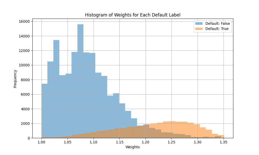
To improve the algorithm’s ability to detect profitable high-risk loans, we will assign greater weight to defaulted loans that resulted in severe losses and, conversely, lower weight to fully paid loans with minimal profits. This approach enhances the model’s ability to distinguish between high-risk, high-return loans and high-risk, low-return loans.

The cost-sensitive model trained with profit-adjusted weights achieves significantly higher profitability, reinforcing that investing in riskier loans with tailored models leads to superior returns.

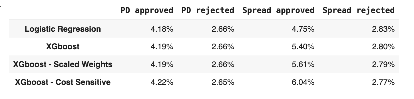Profitability comparison between models and decision threshold.

Conclusion

As Dr. Marcos Lopez de Prado notes in his book Advances in Machine Learning in Finance, many machine learning models struggle in financial applications due to the difficulty of translating real-world complexity into structured learning objectives. However, when tailored correctly—through loss function design, weight adjustments, or cost-sensitive learning —ML models can significantly enhance decision-making and profitability.

I’d love to hear your thoughts, suggestions, and ideas. Thanks for reading!

References

1. Petrides, G. (2022). Cost-sensitive ensemble learning: A unifying framework. Data Mining and Knowledge Discovery.