Or Cohen

Cross Sectional Momentum and Learning to Rank with LambdaMART

In this post, we explore how ranking algorithms—originally developed for search engines—can help us identify winners and losers in investment selection.

There’s an old joke that when your taxi driver tells you to buy a stock, it’s time to sell. This highlights the fact that the diffusion of new information and investors’ responses often lag behind significant price movements. This ripple effect in investors’ reactions leads to autocorrelation in asset returns, reinforcing the persistence of trends—whether upward or downward.

The momentum effect in financial markets dates back as far as the Dutch merchant fleet in 17th-century Amsterdam. Its existence is supported by fundamental economic principles of supply and demand and reflects persistent deviations from market equilibrium.

“An object in motion tends to stay in motion, an object at rest tends to remain at rest.” – Sir Isaac Newton

Time-series momentum (TSM) is identified by analyzing an asset’s own price history, whereas cross-sectional momentum (CSM) is observed by benchmarking an asset’s performance against similar assets. Both can be studied over different time horizons and effectively capture risk premia, challenging the efficient market hypothesis.

A key advantage of the CSM strategy is its ability to hedge against broad market movements (beta) by going long on assets with the highest expected returns and short on those with the lowest. Accurately ranking assets is crucial for optimizing trading performance.

Like any trading strategy, momentum strategies carry unique risks, and overlooking them is a surefire way to lose money. The primary risk to momentum is its counterpart, mean reversion, since trends can reverse sharply. Additionally, momentum strategies perform well in trending markets but struggle in sideways or volatile conditions.

Learning to Rank and LambdaMART

The increasing volume of digital data and the need for efficient search algorithms have driven advances in machine-learned ranking (MLR)—a family of algorithms designed for information retrieval. These models rank search results based on relevance metrics. Learning to rank in search task. Souce: Elastic Search.

One such model is LambdaMART, a state-of-the-art MLR algorithm developed by Christopher J.C. Burges and his colleagues at Microsoft Research [1]. LambdaMART transforms ranking tasks into pairwise classification or regression problems. This means it evaluates pairs of items at a time, determines their optimal ordering, and then combines these comparisons into a final ranking.

LambdaMART’s flexibility makes it a preferred choice for various applications. In ranked search results, it can be optimized for precision, retrieving only the most relevant entries. In financial applications like CSM, maximizing a ranking-specific evaluation metric such as NDCG (Normalized Discounted Cumulative Gain) is more suitable.

The MART component of LambdaMART stands for Multiple Additive Regression Trees, which means the algorithm utilizes gradient boosting with decision trees. Boosting iteratively builds trees, where each new tree corrects errors from previous iterations to optimize ranking metrics such as NDCG or Mean Reciprocal Rank (MRR).

Leveraging MLR for CSM

The advantage of MLR techniques in financial applications stems from their ability to address ranking tasks directly—circumventing the need for standard regression or classification loss functions on returns.

A study by Poh et al. [2] introduced a framework for using MLR to construct CSM portfolios, demonstrating significant performance improvements over traditional ranking techniques. The framework utilizes momentum indicators derived from historical daily prices over 3- to 12-month periods to predict one-month-ahead winners and losers.

One such predictor is the CTA Momentum Indicator, a refined version of the MACD momentum indicator, originally introduced in [3].

CTA Momentum Indicator

This indicator measures trend strength under two assumptions: (1) volatility weakens trend significance, and (2) different assets exhibit unique trend behaviors over time. A robust indicator should account for these variations.

The algorithm for obtaining this signal is the following (as detailed in [3]):

Step 1: Select three time-scale sets, each with a short and long exponentially weighted moving average (EWMA): The authors chose \(S_k = (8, 16, 32)\) and \(L_k = (24, 48, 96).\) Those numbers are not look-back days or half-life numbers. In fact, each number (let’s call it n) translates to a lambda decay factor (\(\lambda\)) to plug into the standard definition of an EWMA. The half-life (HL) is then given by:

Step 2: For each k=1,2,3 calculate:

Step 3: We normalize with a moving standard deviation as a measure of the realized 3-months normal volatility (PW=63):

Step 4: We normalize this series with its realized annual standard deviation (SW=252):

Step 5: We calculate an intermediate signal for each k=1,2,3 via a response function R:

Step 6: The final CTA momentum signal is the weighted sum of the intermediate signals (here we have chosen equal weights \(w_k = \frac{1}{3}\)​):

We can implement it in Python using Pandas broadcasting and vectorization methods which allow efficient computation with fast execution as follows:

hl = lambda decay : np.log(0.5) / np.log(1-1/decay)
macd = lambda S, L: data.Close.ewm(halflife=hl(S)).mean() - 
data.Close.ewm(halflife=hl(L)).mean()

def CTA_momentum(s,l):
	"""
	Computes the signal as defined by Jamil Baz including the
	interim signals for a given set of lambda decay factors
	"""
	phi = []
	result = {}
	for i in zip(s,l):
		y_k = macd(i[0],i[1]) / data.Close.rolling(63).std()
		z_k = y_k / y_k.rolling(252).std()
		result[f'macd_norm_{i}'] = z_k
		u_k = z_k.apply(lambda x: x * np.exp(-(x**2)/4) / 0.89)
		phi.append(u_k)
	result['signal'] = pd.concat(phi ,axis=1).T.groupby(level=0).mean().T
	return pd.concat(result.values(), axis=1, keys=result.keys())
		.resample('ME').last().swaplevel(axis=1).stack(level=0)

Model setup

The framework proposed in [2] uses the CTA momentum signal as well as the normalized MACD signals (ie. the values of \(z_k\)) for the past 1, 3, 6 and 12-months periods along as well as normalized and raw return returns for the past 3, 6 and 12-months periods. We will use log returns for reasons that are explained in this post.

log_prices = data.Close.apply(np.log)
raw_ret = lambda n: log_prices.resample('ME').last().diff(n)
norm_ret = lambda n: log_prices.resample('ME').last().diff(n) / 
	log_prices.diff().ewm(span=n*21).std().resample('ME').last() * np.sqrt(12/n)

All together we get a matrix of 22 features for each stock and month. On a high level this is the process we preform at every rebalance point (month end) :

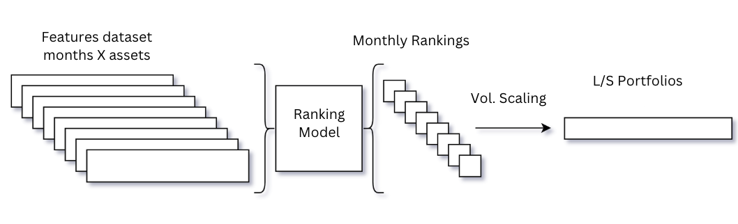
For the ranking objective we’ll use the return achieved over the following month divided to deciles. After we train the model and get the predicted rankings, at each rebalance point (end of each month) the assets at the top and bottom deciles will be added to the portfolio (long and short respectively) scaled by their 3 month exponentially weighted standard deviation. The target annualized standard deviation \(\sigma_{tgt}\) is set to 15%. Expressed formally:

forward_returns = raw_ret(1).shift(-1).stack()
y = pd.DataFrame({
	'forward_return':forward_returns,
	'decile':forward_returns.groupby(level=0) # group by month
	.apply(lambda x: pd.qcut(x, q=10, labels=False, duplicates='drop')).values,
	'risk_weight': (0.15 / log_prices.diff().ewm(span=63).std().resample('ME')
	.last().shift(-1)).stack().reindex(forward_returns.index)
	})

We’ll perform a grid search to find the best set of hyper parameters among those proposed in the research.

param_grid = {
	'eta': [1, 1e-1, 1e-2, 1e-3, 1e-3, 1e-5, 1e-6],
	'n_estimators': [5, 10, 20, 40, 80, 160, 320],
	'max_depth': [2, 4, 6, 8, 10]
	}
param_combinations = [
	dict(zip(param_grid.keys(), v)) for v in product(*param_grid.values())
	]

for params in param_combinations:
	cv_scores = []
	ranker = xgb.XGBRanker(
		objective='rank:pairwise',
		eval_metric='ndcg',
		tree_method='hist',
		eta=params['eta'],
		max_depth=params['max_depth'],
		n_estimators=params['n_estimators'],
		device='cuda'
		)	
		
	ranker.fit(
		X_train, y_train, group=train_group_sizes,
		eval_set=[(X_val, y_val)],
		eval_group=[val_group_sizes],
		verbose=False
		)

With the trained model we can generate monthly predictions and backtest the results to asses its performance.

result = pd.DataFrame(
	index= X_test.index,
	data= ranker.predict(X_test.values), 
	columns=['model_score'])
result['predicted_rank']= result.groupby(level=0)['model_score']
	.apply(lambda x: pd.qcut(x, q=10, labels=False, duplicates='drop')).values

Evaluation

In the research [2] the LambdaMART algorithm was benchmarked with several ranking techniques and models and significantly outperformed. From the figure below which charts the cumulative returns we can clearly notice the advantage of the Learning to Rank methods (LMLE, LNet, LM, and RNet) over traditional ranking methods. 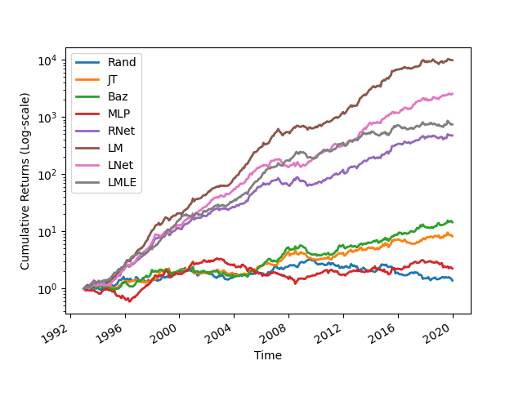Wealth curves rescaled to target volatility. Source: [2]

The reference benchmark models are:

• Random (Rand) – This model select stocks at random, and is included to provide an absolute baseline sense of what the ranking measures might look like assuming portfolios are composed in such a manner.

• Raw returns (JT) – Heuristics-based ranking technique based on [4], which is one of the earliest works documenting the CSM strategy.

• Volatility Normalised MACD (Baz) – Heuristics- based ranking technique with a relatively sophisticated trend estimator proposed by [3].

• Multi-Layer Perceptron (MLP) – This model characterizes the typical Regress-then-rank techniques used by contemporary methods.

• RankNet (RNet) – Pairwise LTR model by [5].

• LambdaMART (LM) – Pairwise LTR model by [1].

• ListNet (LNet) – Listwise LTR model by [6].

• ListMLE (LMLE) – Listwise LTR model by [7].

The following performance metrics taken from [2] solidify the conclusion as it stands out that the LambdaMART algorithm achieved superior performance across all risk adjusted performance metrics (Sharpe, MDD, Sortino, and Calmar). Most noticeable is the average out-of-sample Sharpe ratio of ~2.1 that was acheived with a monthly rebalance frequency. This is quite impressive considering that the test set includes the global financial crisis of 2007. 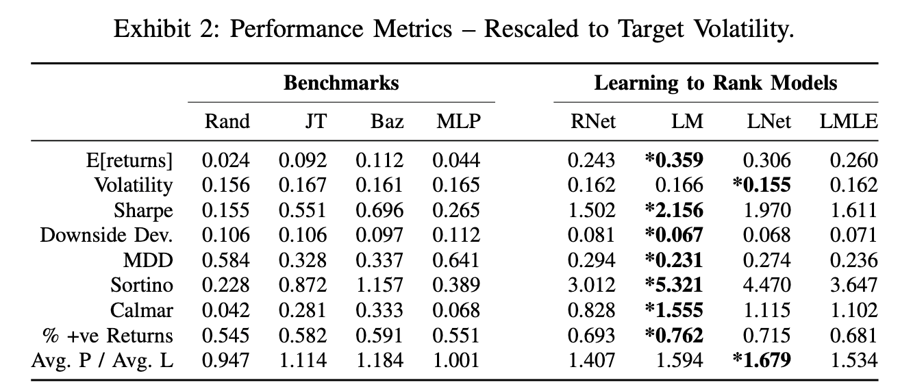Annualized performance metrics. Source: [2]

Conclusion

Momentum is a powerful factor that we can harness to managing our investments and can in fact greatly compliment other factors such as value. We saw how algorithms from another domain can help us with the right methodology and clever predictors.

We can further enhance the ranking accuracy and the financial performance by adding features. For example, relative strength metrics such as Jensen’s alpha will provide the model more (or less) evidence for recent abnormal excess return of a given asset over its peers.

Please don’t hesitate to send any questions or suggestions you have. Thank you for reading!

References:

1. Burges, C (2010). From RankNet to LambdaRank to LambdaMART, Microsoft Research.
2. Poh, D (2020). Building Cross-Sectional Systematic Strategies By Learning to Rank, Oxford-Man Institute of Quantitative Finance.
3. Baz, J. (2015). Dissecting Investment Strategies in the Cross Section and Time Series, SSRN Electronic Journal.
4. Jegadeesh, N. (1993). Returns to Buying Winners and Selling Losers: Implications for Stock Market Efficiency, The Journal of Finance.
5. Burges, C. (2005). Learning to rank using gradient descent, Proceedings of the 22nd International Conference on Machine Learning.
6. Cao, Z. (2007). Learning to rank: From pairwise approach to listwise approach, Proceedings of the 24th International Conference on Machine Learning.
7. Xia, F. (2008). Listwise approach to learning to rank: Theory and algorithm, Proceedings of the 25th International Conference on Machine Learning.